01 Introduction to Shiny

background-image: url("images/title.jpg")
background-size: cover

<ul class="hextile clr">
	<li>
    <div>
      <h1>01</h1>
      <p style = "padding-top: 20%; font-size: 1.5em">Intro to Shiny</p>
    </div>
  </li>
  <li>
    <img src="images/shiny.svg" alt=""/>
  </li>
  <li></li>
  </li>
  <li>
    <div>
      <p style = "padding-top: 20%; font-size: 1.33em">
      Mitchell O'Hara‑Wild
      </p>
    </div>
  </li>
</ul>

.footnote[
Materials at [workshop.mitchelloharawild.com/shiny-basics/](https://workshop.mitchelloharawild.com/shiny-basics/)
]

---
class: left-side

.pull-left.center.bg-blond[

.portrait[
![](images/mitch.jpeg)
]

### Mitchell O'Hara-Wild

### Monash + Nectric

[<svg aria-hidden="true" role="img" viewBox="0 0 496 512" style="height:1em;width:0.97em;vertical-align:-0.125em;margin-left:auto;margin-right:auto;font-size:inherit;fill:currentColor;overflow:visible;position:relative;"><path d="M165.9 397.4c0 2-2.3 3.6-5.2 3.6-3.3.3-5.6-1.3-5.6-3.6 0-2 2.3-3.6 5.2-3.6 3-.3 5.6 1.3 5.6 3.6zm-31.1-4.5c-.7 2 1.3 4.3 4.3 4.9 2.6 1 5.6 0 6.2-2s-1.3-4.3-4.3-5.2c-2.6-.7-5.5.3-6.2 2.3zm44.2-1.7c-2.9.7-4.9 2.6-4.6 4.9.3 2 2.9 3.3 5.9 2.6 2.9-.7 4.9-2.6 4.6-4.6-.3-1.9-3-3.2-5.9-2.9zM244.8 8C106.1 8 0 113.3 0 252c0 110.9 69.8 205.8 169.5 239.2 12.8 2.3 17.3-5.6 17.3-12.1 0-6.2-.3-40.4-.3-61.4 0 0-70 15-84.7-29.8 0 0-11.4-29.1-27.8-36.6 0 0-22.9-15.7 1.6-15.4 0 0 24.9 2 38.6 25.8 21.9 38.6 58.6 27.5 72.9 20.9 2.3-16 8.8-27.1 16-33.7-55.9-6.2-112.3-14.3-112.3-110.5 0-27.5 7.6-41.3 23.6-58.9-2.6-6.5-11.1-33.3 2.6-67.9 20.9-6.5 69 27 69 27 20-5.6 41.5-8.5 62.8-8.5s42.8 2.9 62.8 8.5c0 0 48.1-33.6 69-27 13.7 34.7 5.2 61.4 2.6 67.9 16 17.7 25.8 31.5 25.8 58.9 0 96.5-58.9 104.2-114.8 110.5 9.2 7.9 17 22.9 17 46.4 0 33.7-.3 75.4-.3 83.6 0 6.5 4.6 14.4 17.3 12.1C428.2 457.8 496 362.9 496 252 496 113.3 383.5 8 244.8 8zM97.2 352.9c-1.3 1-1 3.3.7 5.2 1.6 1.6 3.9 2.3 5.2 1 1.3-1 1-3.3-.7-5.2-1.6-1.6-3.9-2.3-5.2-1zm-10.8-8.1c-.7 1.3.3 2.9 2.3 3.9 1.6 1 3.6.7 4.3-.7.7-1.3-.3-2.9-2.3-3.9-2-.6-3.6-.3-4.3.7zm32.4 35.6c-1.6 1.3-1 4.3 1.3 6.2 2.3 2.3 5.2 2.6 6.5 1 1.3-1.3.7-4.3-1.3-6.2-2.2-2.3-5.2-2.6-6.5-1zm-11.4-14.7c-1.6 1-1.6 3.6 0 5.9 1.6 2.3 4.3 3.3 5.6 2.3 1.6-1.3 1.6-3.9 0-6.2-1.4-2.3-4-3.3-5.6-2z"/></svg> @mitchelloharawild](https://github.com/mitchelloharawild)

[<svg aria-hidden="true" role="img" viewBox="0 0 512 512" style="height:1em;width:1em;vertical-align:-0.125em;margin-left:auto;margin-right:auto;font-size:inherit;fill:currentColor;overflow:visible;position:relative;"><path d="M459.37 151.716c.325 4.548.325 9.097.325 13.645 0 138.72-105.583 298.558-298.558 298.558-59.452 0-114.68-17.219-161.137-47.106 8.447.974 16.568 1.299 25.34 1.299 49.055 0 94.213-16.568 130.274-44.832-46.132-.975-84.792-31.188-98.112-72.772 6.498.974 12.995 1.624 19.818 1.624 9.421 0 18.843-1.3 27.614-3.573-48.081-9.747-84.143-51.98-84.143-102.985v-1.299c13.969 7.797 30.214 12.67 47.431 13.319-28.264-18.843-46.781-51.005-46.781-87.391 0-19.492 5.197-37.36 14.294-52.954 51.655 63.675 129.3 105.258 216.365 109.807-1.624-7.797-2.599-15.918-2.599-24.04 0-57.828 46.782-104.934 104.934-104.934 30.213 0 57.502 12.67 76.67 33.137 23.715-4.548 46.456-13.32 66.599-25.34-7.798 24.366-24.366 44.833-46.132 57.827 21.117-2.273 41.584-8.122 60.426-16.243-14.292 20.791-32.161 39.308-52.628 54.253z"/></svg> @mitchoharawild](https://twitter.com/mitchoharawild)

]

.pull-right[
# Welcome, who am I?

- 🎓 Teaches R data skills at Monash University
- 📊 Data consulting and workshops at Nectric
- 📈 Specialised in time series analysis
- 📦 Develops R packages (fable, vitae, etc.)
- 🤖 Makes IoT devices for home automation
- 🐝 Keeps bees, chickens and practices permaculture
]

---
class: left-side

.pull-left.center.bg-blond[

.portrait[
![](images/patrick.jpeg)
]

### Patrick Li

### Monash

]

.pull-right[
# Welcome, who am I?

- 🎓 Second-year PhD student at Monash University
- 🔎 Working on automated visual inference using computer vision models
- 📦 Interested in machine learning, computer vision, data visualisation and statistical software development.
]

---
class: iframe-page

.center[
<https://workshop.mitchelloharawild.com/shiny-basics/>
]

---
class: bg-yellow feature

# 🎯 Tutorial goals

.box-12.larger[
1.  **Learn the basics** of Shiny applications
1.  Create a simple **user interface** including dashboards
1.  Understand **reactive programming** for Shiny server code
1.  **Publish applications** online with docker and/or [shinyapps.io](https://www.shinyapps.io/)
]

# 🎁 Tutorial apps

```r
usethis::use_course("https://workshop.mitchelloharawild.com/apps.zip")
```

---
class: bg-yellow feature

# ✅ Expectations

.box-12.larger[
* **Respect** each other
* **Engage** by attempting exercises and asking questions
* **Learn** the basics of shiny!
]

# ❓ Questions

.box-12.larger[
* **Interrupt** for relevant questions
* **Wait** for exercises/break for off-topic questions
* **Introduce** yourself with one interest (job, hobby, anything!)
* **Ask** with your microphone, or use chat if you prefer.
]

---

class: left-side

.pull-left.center.bg-blond[

# What is Shiny?

.sticker-left[![shiny](images/shiny.svg)]

]

.pull-right[
> Shiny is a framework for creating web applications using R code.
>
> [*Mastering Shiny*](https://mastering-shiny.org/)
]

.pull-right[
Shiny allows you to:

* Interactively explore data
* Use R code to perform analysis for web users
* Quickly & easily produce sophisticated apps
]

---

# I use shiny to...

1. Rapidly produce useful tools for the web
1. Allow non-programmers to use powerful R packages
1. Produce interactive learning experiences
1. Create dashboards for data management

.box-12.bg-blond[
In the eyes of most people, quickly creating a shiny app is magic ✨🧙‍♂️.
]

---
background-image: url("images/hive_ss.png")
background-size: contain
background-position: top

.box-12.bg-blond.bottom-margin.center[
# Visualise native Australian bee sightings
<https://shiny.mitchelloharawild.com/hive/>
]

---
background-image: url("images/fpp3_ss.png")
background-size: contain
background-position: top

.box-12.bg-blond.bottom-margin.center[
# Teach statistical concepts
<https://otexts.com/fpp3/prediction-intervals.html>
]

---
background-image: url("images/cooee_ss.png")
background-size: contain
background-position: top

.box-12.bg-blond.bottom-margin.center[
# Simplify evaluation of abstract submissions
<https://github.com/useR-2018/cooee>
]

---
background-image: url("images/taipan_ss.png")
background-size: cover

.sticker-float[![](images/taipan.png)]

.box-12.bg-blond.bottom-margin.center[
# Train & validate machine learning models
<https://srkobakian.github.io/taipan/>
]

---

# Basic components of a shiny app

```r
library(shiny)
ui <- fluidPage(
  "Hello, world!"
)
server <- function(input, output, session) {
  # Nothing to see here!
  # All this app does is say "Hello, world!"
}
shinyApp(ui, server)
```

The simplest app consists of a **UI** and **server**, in a single file: `app.R`.

- The UI controls the layout, style and interactivity (HTML, CSS, JS)
- The server controls the behaviour (R)

The glue that holds it together is JavaScript and WebSockets.

Shiny allows you to do everything with **only** R code!

---
class: feature

# 🌠 Your turn!

.box-12[

## Starter shiny app 🔍

Run the 'Hello World!' app using code from the previous slide.

1. Copy the code into a new `app.R` file
1. Launch the app using the **Run App** button ![button](images/run_app.png)
1. Close the app using the stop button 🛑

]

---
class: center

# Where does this app live?

```r
runApp('hello_world')

#> Listening on http://127.0.0.1:5545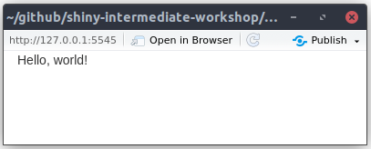
```
![App screenshot](images/hello_world_ss.png)

## 💻 On the web? 🌐

Well, sort of! When running an app locally, your computer serves the app at a local address (`127.0.0.1` or `localhost`).

More on this in session 3!

---
class: center

# View the app in a web browser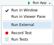

![Run external](images/run_app_external.png)

When an app is ran locally, it is only accessible to you.

Deploying the app on a server allows others access the app without R.

---

# Adding inputs to the UI

Inputs allow users to provide information to control the app.

**UI**: All **inputs** functions follow a similar signature:

```r
textInput(
  inputId = "input_user_text", # ID to obtain text in server code
  label = "Display label", # Guide the user with what to input
  value = "Default text" # Initial value in the box
)
```

<div class="form-group shiny-input-container">
<label class="control-label" id="input_user_text-label" for="input_user_text">Display label</label>
<input id="input_user_text" type="text" class="form-control" value="Default text"/>
</div>

**Server**: The provided text for this box is accessible in the server code with:

```r
input$input_user_text # The provided inputId
```

<div class="remark-code-line"><code id="output_server_text" class="remark-code remark-inline-code">## [1] "Default text"</code></div>

---

# Adding outputs to the UI

Outputs return information from the server to the interface.

**UI**: All **output** functions also have similar arguments:

```r
textOutput(
  outputId = "output_server_text", # ID used by server code
)
```

<div id="output_server_text" class="shiny-text-output"></div>
My text from the server!

**Server**: The server provides output to the UI using **render** functions:

```r
output$output_server_text <- renderText({
  "My text from the server!"
  # You could use any R code here, perhaps even inputs like input$input_user_text
})
```

---
class: feature

# 🌠 Your turn!

.box-12[

## Hello you!

Extend the 'Hello World!' app to greet the user's name, rather than 'world'.

1. Add a text input field to provide the user's name.
1. Replace the static 'Hello World!' text with a text output.
1. Add a text renderer to the server, which creates the output 'Hello {{name}}!'

If you have time, modify the app to say 'Good morning', 'Good afternoon' and 'Good night' based on `Sys.time()`

]

---

# ⛳ Possible solution

```r
library(shiny)
ui <- fluidPage(
  textInput("name", "Enter your name: "),
  textOutput("greeting")
)
server <- function(input, output, session) {
  output$greeting <- renderText({
    sprintf("Hello %s!", input$name)
  })
}
shinyApp(ui, server)
```

### Bonus:

```r
output$greeting <- renderText({
  hour <- lubridate::hour(Sys.time())
  time <- if (dplyr::between(hour, 6, 11)) "morning" else
          if (dplyr::between(hour, 12, 18)) "afternoon" else "night"
  sprintf("Good %s %s!", time, input$name)
})
```

---
background-image: url("images/cheatsheet.png")
background-size: contain
background-position: top

.box-12.bg-blond.bottom-margin.center[
# 📖 Shiny cheatsheet 📖
# (Inputs and outputs galore)
https://shiny.rstudio.com/images/shiny-cheatsheet.pdf
]

---

# A multi-file shiny app

```r
fs::dir_tree("../apps/bob_ross/01_bob_ross")
```

```
## ../apps/bob_ross/01_bob_ross
## ├── data
## │   └── elements-by-episode.csv
## ├── global.R
## ├── server.R
## ├── ui.R
## └── www
##     └── joy_of_painting.jpg
```

Most shiny apps are organised into several files.

* `ui.R`: The specification of the user interface
* `server.R`: The R code to define behaviour
* `global.R`: Objects creation accessible to both `ui.R` and `server.R`
* `data/`: Folder for your data
* `www/`: Folder for your web data (images, css, javascript, etc.)

---
background-image: url("images/bob_ross.png")
background-size: contain
background-position: top

.box-12.bg-blond.bottom-margin.center[
# 🎨 A happy little app 🎨
A shiny app for FiveThirtyEight's [*Statistical Analysis of the Work of Bob Ross*](https://fivethirtyeight.com/features/a-statistical-analysis-of-the-work-of-bob-ross/)

Try the app for yourself, you can find it in "bob_ross/01_bob_ross".
]

---

# 🌏 `global.R`: Global objects

```r
library(tidyverse)

# Tidy the data
elements <- read_csv("data/elements-by-episode.csv") %>% 
  separate(EPISODE, c("season", "episode"), sep = c(3,6)) %>% 
  gather("element", "exists", -season, -episode, -TITLE) %>% 
  mutate(
    season = parse_number(season),
    episode = parse_number(episode),
    element = str_to_sentence(str_replace_all(element, "_", " ")),
    TITLE = str_to_sentence(TITLE),
    exists = as.logical(exists)
  ) %>% 
  rename(title = TITLE)
```

---

# 🎨 `ui.R`: Understanding the UI

```r
library(shiny)
fluidPage(
  titlePanel("Bob Ross painting contents"),
  sidebarLayout(
    sidebarPanel(
      # Joy of painting title image
      img(src = "joy_of_painting.jpg", width = "100%"),
      # Season selector
      sliderInput(inputId = "seasons",
                  label = "Included seasons:",
                  min = min(elements$season),
                  max = max(elements$season),
                  value = range(elements$season))
    ),
    mainPanel(
      # Plot output
      "Frequency of elements in paintings",
      plotOutput(outputId = "plot_proportion", height = "800px"),
      # Table output
      "Top 10 most common elements",
      tableOutput(outputId = "data_proportion")
    )
  )
)
```

---

# 🎨 `ui.R`: A two-panel sidebar layout

```r
library(shiny)
fluidPage(
  titlePanel("Bob Ross painting contents"),
* sidebarLayout(
*   sidebarPanel(
      # Joy of painting title image
      img(src = "joy_of_painting.jpg", width = "100%"),
      # Season selector
      sliderInput(inputId = "seasons",
                  label = "Included seasons:",
                  min = min(elements$season),
                  max = max(elements$season),
                  value = range(elements$season))
*   ),
*   mainPanel(
      # Plot output
      "Frequency of elements in paintings",
      plotOutput(outputId = "plot_proportion", height = "800px"),
      # Table output
      "Top 10 most common elements",
      tableOutput(outputId = "data_proportion")
*   )
* )
)
```

---

# 🎨 `ui.R`: Add an image from `www` folder

```r
library(shiny)
fluidPage(
  titlePanel("Bob Ross painting contents"),
  sidebarLayout(
    sidebarPanel(
*     # Joy of painting title image
*     img(src = "joy_of_painting.jpg", width = "100%"),
      # Season selector
      sliderInput(inputId = "seasons",
                  label = "Included seasons:",
                  min = min(elements$season),
                  max = max(elements$season),
                  value = range(elements$season))
    ), 
    mainPanel(
      # Plot output
      "Frequency of elements in paintings",
      plotOutput(outputId = "plot_proportion", height = "800px"),
      # Table output
      "Top 10 most common elements",
      tableOutput(outputId = "data_proportion")
    ) 
  )
)
```

---

# 🎨 `ui.R`: Add the season slider

```r
library(shiny)
fluidPage(
  titlePanel("Bob Ross painting contents"),
  sidebarLayout(
    sidebarPanel(
      # Joy of painting title image
      img(src = "joy_of_painting.jpg", width = "100%"),
*     # Season selector
*     sliderInput(inputId = "seasons",
*                 label = "Included seasons:",
*                 min = min(elements$season),
*                 max = max(elements$season),
*                 value = range(elements$season))
    ), 
    mainPanel(
      # Plot output
      "Frequency of elements in paintings",
      plotOutput(outputId = "plot_proportion", height = "800px"),
      # Table output
      "Top 10 most common elements",
      tableOutput(outputId = "data_proportion")
    ) 
  )
)
```

---

# 🎨 `ui.R`: Add outputs to the main panel

```r
library(shiny)
fluidPage(
  titlePanel("Bob Ross painting contents"),
  sidebarLayout(
    sidebarPanel(
      # Joy of painting title image
      img(src = "joy_of_painting.jpg", width = "100%"),
      # Season selector
      sliderInput(inputId = "seasons",
                  label = "Included seasons:",
                  min = min(elements$season),
                  max = max(elements$season),
                  value = range(elements$season))
    ), 
    mainPanel(
*     # Plot output
*     "Frequency of elements in paintings",
*     plotOutput(outputId = "plot_proportion", height = "800px"),
*     # Table output
*     "Top 10 most common elements",
*     tableOutput(outputId = "data_proportion")
    ) 
  )
)
```

---

# 💻 `server.R`: Creating interactive behaviour

```r
library(shiny)
library(tidyverse)
function(input, output, session) {
  output$plot_proportion <- renderPlot({
    elements_prop <- elements %>% 
      filter(between(season, input$seasons[1], input$seasons[2])) %>% 
      group_by(element) %>% 
      summarise(proportion = mean(exists)) %>% 
      arrange(desc(proportion)) %>% 
      mutate(element = fct_reorder(element, proportion))
    elements_prop %>% 
      ggplot(aes(x = proportion, y = element)) + 
      geom_col() +
      scale_x_continuous(labels = scales::percent, limits = c(0,1))
  })
  output$data_proportion <- renderTable({
    elements %>% 
      filter(between(season, input$seasons[1], input$seasons[2])) %>% 
      group_by(element) %>% 
      summarise(proportion = mean(exists)) %>% 
      arrange(desc(proportion)) %>% 
      mutate(element = fct_reorder(element, proportion)) %>% 
      top_n(10, proportion)
  })
}
```

```
## function(input, output, session) {
##   output$plot_proportion <- renderPlot({
##     elements_prop <- elements %>% 
##       filter(between(season, input$seasons[1], input$seasons[2])) %>% 
##       group_by(element) %>% 
##       summarise(proportion = mean(exists)) %>% 
##       arrange(desc(proportion)) %>% 
##       mutate(element = fct_reorder(element, proportion))
##     elements_prop %>% 
##       ggplot(aes(x = proportion, y = element)) + 
##       geom_col() +
##       scale_x_continuous(labels = scales::percent, limits = c(0,1))
##   })
##   output$data_proportion <- renderTable({
##     elements %>% 
##       filter(between(season, input$seasons[1], input$seasons[2])) %>% 
##       group_by(element) %>% 
##       summarise(proportion = mean(exists)) %>% 
##       arrange(desc(proportion)) %>% 
##       mutate(element = fct_reorder(element, proportion)) %>% 
##       top_n(10, proportion)
##   })
## }
```

---

# 💻 `server.R`: Render to an output

```r
library(shiny)
library(tidyverse)
function(input, output, session) {
* output$plot_proportion <- renderPlot({
    elements_prop <- elements %>% 
      filter(between(season, input$seasons[1], input$seasons[2])) %>% 
      group_by(element) %>% 
      summarise(proportion = mean(exists)) %>% 
      arrange(desc(proportion)) %>% 
      mutate(element = fct_reorder(element, proportion))
    elements_prop %>% 
      ggplot(aes(x = proportion, y = element)) + 
      geom_col() +
      scale_x_continuous(labels = scales::percent, limits = c(0,1))
  })
* output$data_proportion <- renderTable({
    elements %>% 
      filter(between(season, input$seasons[1], input$seasons[2])) %>% 
      group_by(element) %>% 
      summarise(proportion = mean(exists)) %>% 
      arrange(desc(proportion)) %>% 
      mutate(element = fct_reorder(element, proportion)) %>% 
      top_n(10, proportion)
  })
}
```

```
## function(input, output, session) {
##   output$plot_proportion <- renderPlot({ #<<
##     elements_prop <- elements %>% 
##       filter(between(season, input$seasons[1], input$seasons[2])) %>% 
##       group_by(element) %>% 
##       summarise(proportion = mean(exists)) %>% 
##       arrange(desc(proportion)) %>% 
##       mutate(element = fct_reorder(element, proportion))
##     elements_prop %>% 
##       ggplot(aes(x = proportion, y = element)) + 
##       geom_col() +
##       scale_x_continuous(labels = scales::percent, limits = c(0,1))
##   })
##   output$data_proportion <- renderTable({ #<<
##     elements %>% 
##       filter(between(season, input$seasons[1], input$seasons[2])) %>% 
##       group_by(element) %>% 
##       summarise(proportion = mean(exists)) %>% 
##       arrange(desc(proportion)) %>% 
##       mutate(element = fct_reorder(element, proportion)) %>% 
##       top_n(10, proportion)
##   })
## }
```

---

# 💻 `server.R`: Filter based on slider inputs

```r
library(shiny)
library(tidyverse)
function(input, output, session) {
  output$plot_proportion <- renderPlot({
*   elements_prop <- elements %>%
*     filter(between(season, input$seasons[1], input$seasons[2])) %>%
      group_by(element) %>% 
      summarise(proportion = mean(exists)) %>% 
      arrange(desc(proportion)) %>% 
      mutate(element = fct_reorder(element, proportion))
    elements_prop %>% 
      ggplot(aes(x = proportion, y = element)) + 
      geom_col() +
      scale_x_continuous(labels = scales::percent, limits = c(0,1))
  })
  output$data_proportion <- renderTable({
*   elements %>%
*     filter(between(season, input$seasons[1], input$seasons[2])) %>%
      group_by(element) %>% 
      summarise(proportion = mean(exists)) %>% 
      arrange(desc(proportion)) %>% 
      mutate(element = fct_reorder(element, proportion)) %>% 
      top_n(10, proportion)
  })
}
```

```
## function(input, output, session) {
##   output$plot_proportion <- renderPlot({
##     elements_prop <- elements %>% #<<
##       filter(between(season, input$seasons[1], input$seasons[2])) %>% #<<
##       group_by(element) %>% 
##       summarise(proportion = mean(exists)) %>% 
##       arrange(desc(proportion)) %>% 
##       mutate(element = fct_reorder(element, proportion))
##     elements_prop %>% 
##       ggplot(aes(x = proportion, y = element)) + 
##       geom_col() +
##       scale_x_continuous(labels = scales::percent, limits = c(0,1))
##   })
##   output$data_proportion <- renderTable({
##     elements %>% #<<
##       filter(between(season, input$seasons[1], input$seasons[2])) %>% #<<
##       group_by(element) %>% 
##       summarise(proportion = mean(exists)) %>% 
##       arrange(desc(proportion)) %>% 
##       mutate(element = fct_reorder(element, proportion)) %>% 
##       top_n(10, proportion)
##   })
## }
```

---

# 💻 `server.R`: Compute and order by proportion

```r
library(shiny)
library(tidyverse)
function(input, output, session) {
  output$plot_proportion <- renderPlot({
    elements_prop <- elements %>% 
      filter(between(season, input$seasons[1], input$seasons[2])) %>% 
*     group_by(element) %>%
*     summarise(proportion = mean(exists)) %>%
*     arrange(desc(proportion)) %>%
*     mutate(element = fct_reorder(element, proportion))
    elements_prop %>% 
      ggplot(aes(x = proportion, y = element)) + 
      geom_col() +
      scale_x_continuous(labels = scales::percent, limits = c(0,1))
  })
  output$data_proportion <- renderTable({
    elements %>% 
      filter(between(season, input$seasons[1], input$seasons[2])) %>% 
*     group_by(element) %>%
*     summarise(proportion = mean(exists)) %>%
*     arrange(desc(proportion)) %>%
*     mutate(element = fct_reorder(element, proportion)) %>%
      top_n(10, proportion)
  })
}
```

```
## function(input, output, session) {
##   output$plot_proportion <- renderPlot({
##     elements_prop <- elements %>% 
##       filter(between(season, input$seasons[1], input$seasons[2])) %>% 
##       group_by(element) %>%  #<<
##       summarise(proportion = mean(exists)) %>%  #<<
##       arrange(desc(proportion)) %>%  #<<
##       mutate(element = fct_reorder(element, proportion)) #<<
##     elements_prop %>% 
##       ggplot(aes(x = proportion, y = element)) + 
##       geom_col() +
##       scale_x_continuous(labels = scales::percent, limits = c(0,1))
##   })
##   output$data_proportion <- renderTable({
##     elements %>% 
##       filter(between(season, input$seasons[1], input$seasons[2])) %>% 
##       group_by(element) %>%  #<<
##       summarise(proportion = mean(exists)) %>% #<<
##       arrange(desc(proportion)) %>%  #<<
##       mutate(element = fct_reorder(element, proportion)) %>% #<<
##       top_n(10, proportion)
##   })
## }
```

---

# 💻 `server.R`: Create the output

```r
library(shiny)
library(tidyverse)
function(input, output, session) {
  output$plot_proportion <- renderPlot({ 
    elements_prop <- elements %>% 
      filter(between(season, input$seasons[1], input$seasons[2])) %>% 
      group_by(element) %>% 
      summarise(proportion = mean(exists)) %>% 
      arrange(desc(proportion)) %>% 
      mutate(element = fct_reorder(element, proportion))
*   elements_prop %>%
*     ggplot(aes(x = proportion, y = element)) +
*     geom_col() +
*     scale_x_continuous(labels = scales::percent, limits = c(0,1))
  })
  output$data_proportion <- renderTable({ 
    elements %>% 
      filter(between(season, input$seasons[1], input$seasons[2])) %>% 
      group_by(element) %>% 
      summarise(proportion = mean(exists)) %>% 
      arrange(desc(proportion)) %>% 
      mutate(element = fct_reorder(element, proportion)) %>% 
*     top_n(10, proportion)
  })
}
```

```
## function(input, output, session) {
##   output$plot_proportion <- renderPlot({ 
##     elements_prop <- elements %>% 
##       filter(between(season, input$seasons[1], input$seasons[2])) %>% 
##       group_by(element) %>% 
##       summarise(proportion = mean(exists)) %>% 
##       arrange(desc(proportion)) %>% 
##       mutate(element = fct_reorder(element, proportion))
##     elements_prop %>% #<<
##       ggplot(aes(x = proportion, y = element)) + #<<
##       geom_col() +#<<
##       scale_x_continuous(labels = scales::percent, limits = c(0,1))#<<
##   })
##   output$data_proportion <- renderTable({ 
##     elements %>% 
##       filter(between(season, input$seasons[1], input$seasons[2])) %>% 
##       group_by(element) %>% 
##       summarise(proportion = mean(exists)) %>% 
##       arrange(desc(proportion)) %>% 
##       mutate(element = fct_reorder(element, proportion)) %>% 
##       top_n(10, proportion) #<<
##   })
## }
```

---
class: center

.box-12.bg-blond[
# 🚧 This app has room for improvement! 🚧
]

# How could we make it better?

Remove code duplication

Add comments to server code

Make it more useful

Improve layout of outputs

Make it look better

---
class: center

.box-12.bg-blond[
# 🚧 This app has room for improvement! 🚧
]

# How could we make it better?

Remove code duplication

Add comments to server code

**Make it more useful**

**Improve layout of outputs**

Make it look better

---

# 📊 Improving the layout of outputs with tabs

```r
tabsetPanel( 
  tabPanel("Plot", 
    "Frequency of elements in paintings",
    plotOutput("plot_proportion", height = "800px")
  ), 
  tabPanel("Table", 
    # Table output
    "Top 10 most common elements",
    tableOutput("data_proportion")
  )
)
```

.center[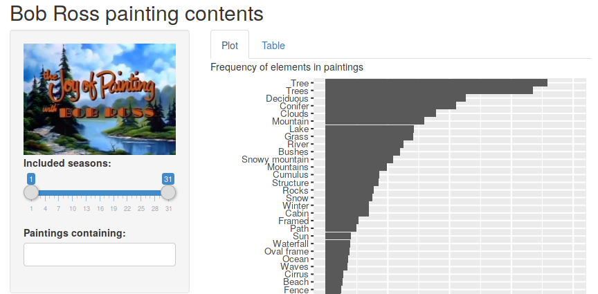
![](images/ross_tabs.png)
]

---
class: feature

# 🌠 Your turn!

.box-12[
## Make the app more useful! 👨‍🎨 👩‍🎨
.center[
![](images/ross.gif)
]
]

---
class: feature

# 🌠 Your turn!

.box-12[
## Make the app more useful! 👨‍🎨 👩‍🎨

Add a selectize input (`selectizeInput()`) which allows you to focus on paintings which contain specific elements.

The output plot and table should show element frequency of paintings which:
* Are in the selected season(s)
* Contain the selected elements

Speedster? There's no need to show 100% frequencies for the selected elements, remove them from the outputs.

]

---

# ⛳ Possible solution

### `ui.R`

```r
# Element selector
selectizeInput("elements",
               "Paintings containing:",
               choices = unique(elements$element),
               multiple = TRUE)
```

### `server.R`

```r
elements %>% 
* group_by(season, episode) %>%
* filter(all(input$elements %in% element[exists])) %>%
  filter(between(season, input$seasons[1], input$seasons[2])) %>% 
  ...
```

### Bonus

```r
... %>% 
  filter(!(element %in% input$elements))
```

---
class: feature

# 🏁 Extra time?

.box-12[
## Work on your own app

If you haven't brought an app today, create one for your script.

If you already have an app:
1. Can you add inputs to make it more useful?
1. Is the layout well organised for the user?
1. Could you improve your app with a picture?

]

---
class: feature

# 🕥 Break time!

.box-12[
## Next topic: reactivity 💥

Time for a break! Take some time to practice shiny by making an app or modifying the examples shown. Ask questions, or just relax and ready yourself to learn about reactive programming!

![reactlog](images/reactivity.gif)
]